planets-princomp.sagews

Метод главных компонент

%r
planets <- read.table('planets.csv', header=TRUE, sep=",")
planets.pca <- princomp(scale(planets[, 2:5]))
plot(planets.pca)

%r
# Похоже, что у нас две главные компоненты... Проверим!
summary(planets.pca)

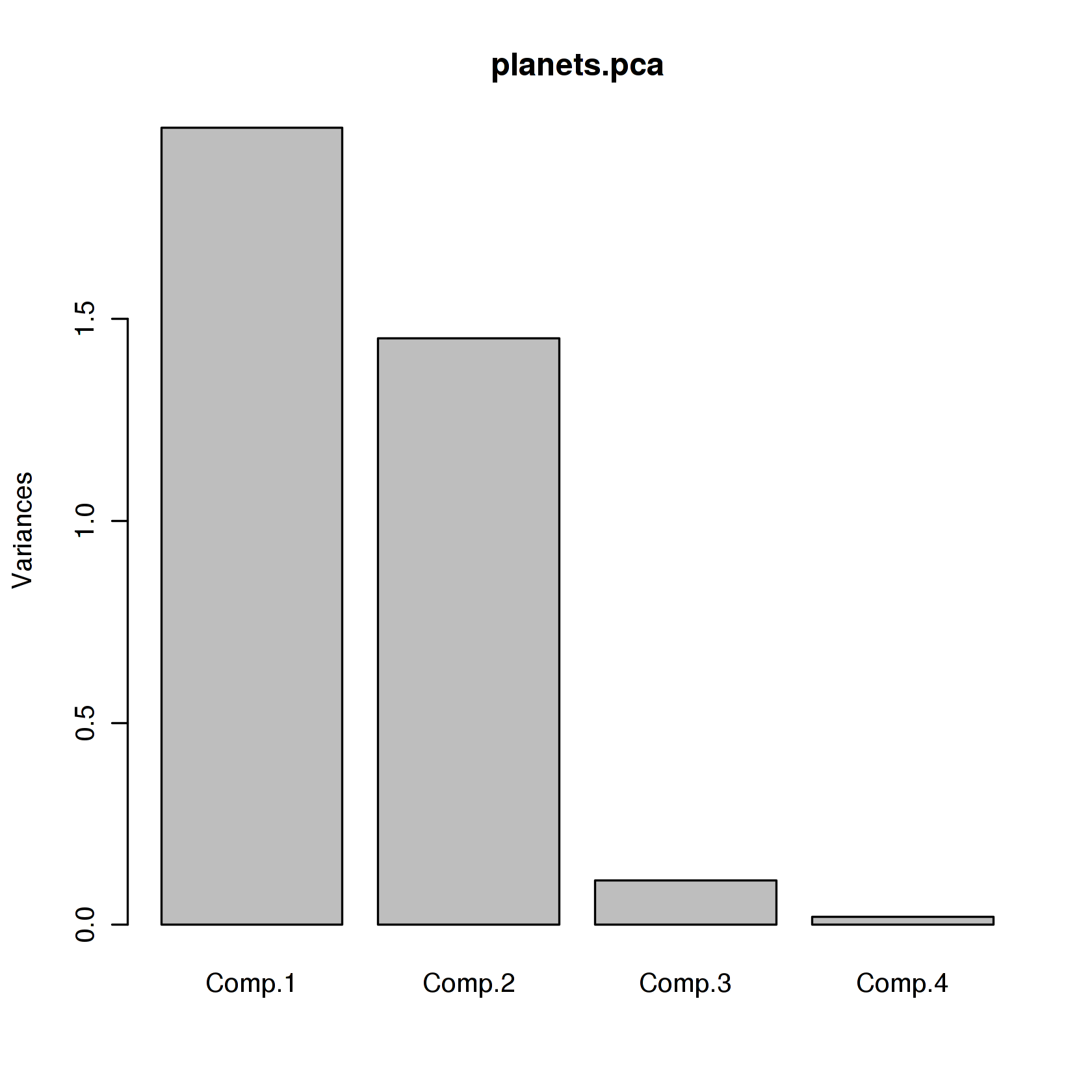
Importance of components: Comp.1 Comp.2 Comp.3 Comp.4 Standard deviation 1.4046031 1.2051824 0.33257821 0.139902076 Proportion of Variance 0.5548809 0.4085057 0.03110858 0.005504791 Cumulative Proportion 0.5548809 0.9633866 0.99449521 1.000000000

%r
# Но что это за компоненты?..
loadings(planets.pca)

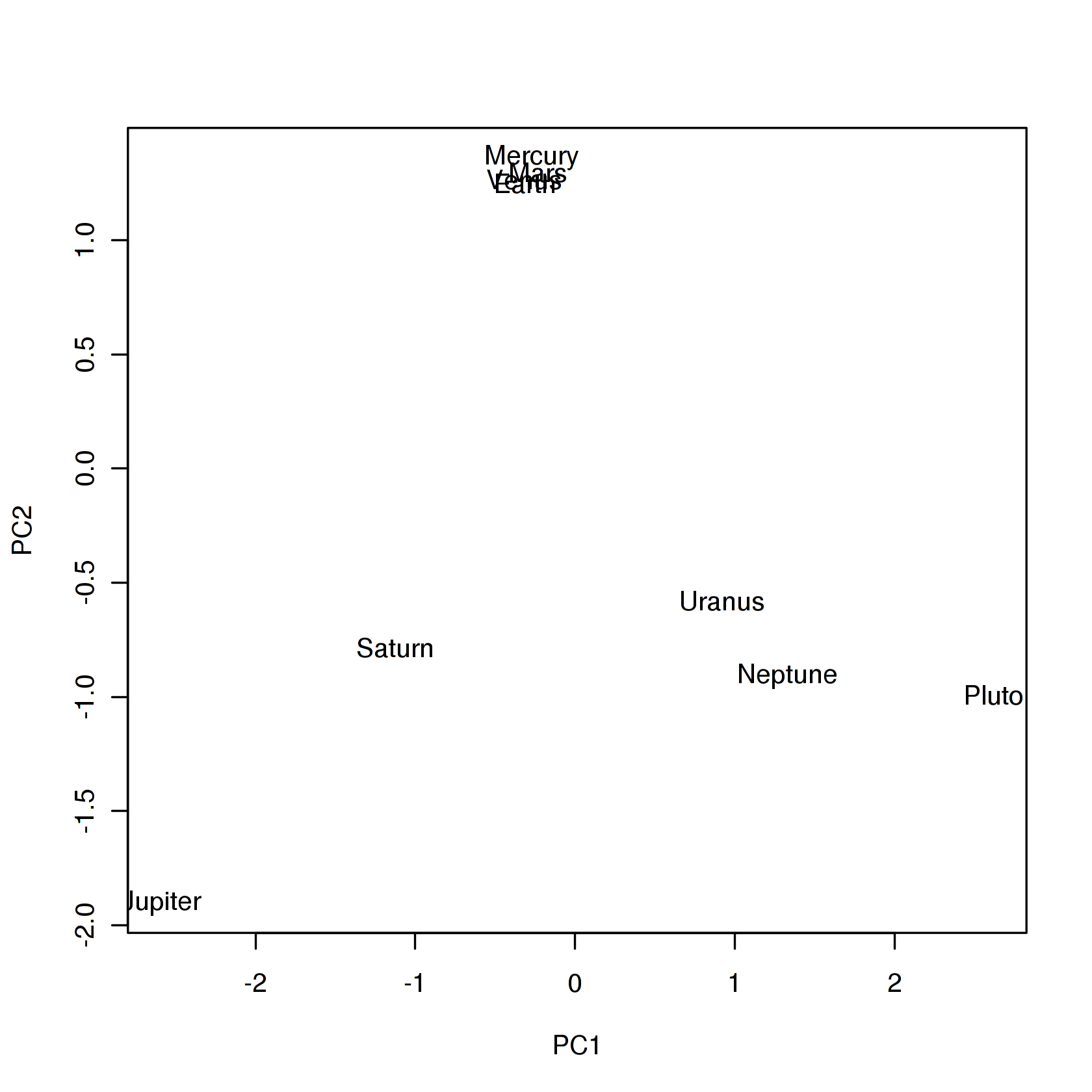
Loadings: Comp.1 Comp.2 Comp.3 Comp.4 Distance 0.527 -0.477 -0.703 Diameter -0.424 -0.575 -0.698 Period 0.559 -0.424 0.709 Mass -0.479 -0.512 0.713 Comp.1 Comp.2 Comp.3 Comp.4 SS loadings 1.00 1.00 1.00 1.00 Proportion Var 0.25 0.25 0.25 0.25 Cumulative Var 0.25 0.50 0.75 1.00

%r
planets.p <- predict(planets.pca)
plot(planets.p[, 1:2], type="n", xlab="PC1", ylab="PC2")
text(planets.p[, 1:2], labels=planets[, 1])